功能描述:
function varargout = legendrefit(Y, N, method)
%LEGENDREFIT Fitting data using a linear combination of Legendre polynomials
%
% A = legendrefit(Y, N, method) finds the column vector A which contains
% weighting coefficients of the linear combination of a set of Legendre
% polynomials up to order N. A(i) is the weight of P_{i-1}(x) which is
% Legendre polynomial of order i-1. The fitting is optimum in the least
% squares sense. If N is not specified, default order 2 is used.
%
% Three methods are available (just for fun): 'inv' (default) inverts the
% normal equation matrix directly, while 'chol' and 'qr' find the solution
% via Cholesky and QR decomposition, respectively.
%
% [A Y2] = legendrefit(...) returns the fitting (regression) result Y2,
% i.e. Y2 = \sum_{i=1}^{N+1} A(i)*P_{i-1}(x). Residuals are then Y - Y2.
%
% [A Y2 r] = legendrefit(...) and [A Y2 r e] = legendrefit(...) further
% return the Pearson's correlation coefficient r and root mean square
% error (RMSE) e, respectively.
%
% If no output argument is specified, legendrefit(...) plots the Y and Y2.
%
error(nargchk(1,3,nargin)) % check the number of arguments
error(nargoutchk(0,4,nargout))
% make sure Y is a vector
if all(size(Y)>1)
error('Input data should be a vector.')
end
% check N
if nargin < 2
fprintf('Order N is not specified. Default order N=2 is used.\n')
N = 2; % set N to default
end
if (N < 0 || round(N) ~= N)
fprintf('Input N=%g is not valid. Default order N=2 is used.\n', N)
N = 2;
end
% default method for finding the solution in least squares sense
if nargin < 3
method = 'inv';
end
%%% compute the Legendre polynomial coefficients matrix coeff
% coeff(i,j) gives the polynomial coefficient for term x^{j-1} in P_{i-1}(x)
if N > 1
coeff = zeros(N+1);
coeff([1 N+3]) = 1; % set coefficients of P_0(x) and P_1(x)
% now compute for higher order: nP_n(x) = (2n-1)xP_{n-1}(x) - (n-1)P_{n-2}(x)
for ii = 3:N+1
coeff(ii,:) = (2-1/(ii-1))*coeff(ii-1,[end 1:end-1]) - (1-1/(ii-1))*coeff(ii-2,:);
end
else
% simple case
coeff = eye(N+1);
end
m = length(Y);
X = -1:2/(m-1):1; % Legendre polynomials are supported for |x|<=1
Y = Y(:); % make it a column
X = X(:);
%%% Evaluate the polynomials for every element in X
D = cumprod([ones(m,1) X(:,ones(1,N))], 2) * coeff.';
% or D = cumprod([ones(m,1) repmat(X,[1 N])], 2) * coeff.';
%%% Alternatively, you can compute D as following (slower)
% coeff = coeff(:,end:-1:1); % rearrange the coefficients matrix
% D = zeros(m, N+1);
% for ii = 1:N+1
% D(:,ii) = polyval(coeff(ii,:),X);
% end
%%% Find weighting coefficients for the linear combination of polynomials
switch method
case 'inv'
% Solution 1 (default)
% for ill-conditioned case, method 'qr' may be a better choice
A = (D.'*D)\(D.'*Y); % inverting the normal equations matrix directly
case 'chol'
% Solution 2: Cholesky decomposition
% let D.'*D = R.'*R where R is an upper triangular matrix
% D.'*D should be positive definite
R = chol(D.'*D);
Z = R.'\(D.'*Y);
A = R\Z;
case 'qr'
% Solution 3: QR decomposition
% this method is computionally more intensive, but usually gives
% better numerical stablility
[Q,R] = qr(D,0);
A = R\(Q.'*Y);
otherwise
error('Unknown method! Available methods: ''inv'' (default), ''chol'' and ''qr''.')
end
% fitting (regression) result
Y2 = D*A;
%%% Compute some numerical indicators of how well the fitting is
% Pearson's correlation coefficient
a = Y-mean(Y);
b = Y2-mean(Y2);
r = a.'*b / sqrt((a.'*a)*(b.'*b));
% root mean square error (RMSE)
Z = Y-Y2; % residuals
e = sqrt(Z.'*Z/m);
% e2 = norm(Z); % e = e2/sqrt(m);
%%% allocate outputs
switch nargout
case {1}
varargout = {A};
case {2}
varargout = {A, Y2};
case {3}
varargout = {A, Y2, r};
case {4}
varargout = {A, Y2, r, e};
case{0}
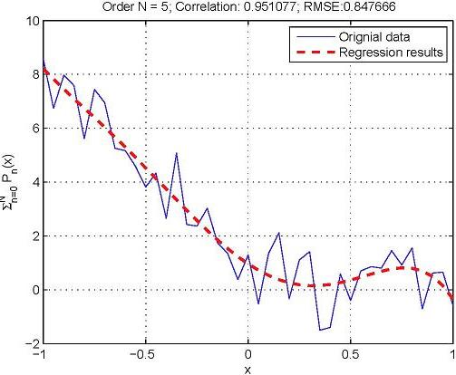
% no output specified, plot Y and Y2
figure, plot(X,Y), grid on
hold on, plot(X,Y2,'--r','linewidth',2)
title(sprintf('Order N = %d; Correlation: %g; RMSE:%g', N, r, e));
xlabel('x'), ylabel('\Sigma_{n=0}^{N} P_n(x)');
legend('Orignial data','Regression results');
end
联系:highspeedlogic
QQ :1224848052
微信:HuangL1121
邮箱:1224848052@qq.com
网站:http://www.mat7lab.com/
网站:http://www.hslogic.com/
微信扫一扫: